Machine learning warm-up

Overfitting occurs when a model fits the training data too closely, including noise or spurious patterns that do not generalize to new data. As a result, the model achieves very low training error but performs poorly on unseen data, such as validation or test data.

A common sign of overfitting is a large gap between training performance and validation performance. For example, the training loss may continue to decrease while the validation loss starts to increase.

Typical ways to reduce overfitting include:

1. cross-validation for model selection;
2. add regularization, such as $L^1$ or $L^2$ penalties (weight decay);
3. reduce model complexity or performing feature selection;
4. increase the amount of training data or using data augmentation;
5. early stopping;
6. ensemble methods.

Underfitting occurs when a model is too simple or too constrained to capture the underlying patterns in the data. As a result, it performs poorly even on the training set, and also generalizes poorly to validation or test data.

A common sign of underfitting is that both the training error and the validation error remain high. In this case, the model has not learned enough structure from the data.

Typical ways to reduce underfitting include:

1. increase model complexity;
2. add more informative features;
3. reduce regularization strength;
4. train for more iterations or epochs.

Suppose the true relationship is$y = f(x) + \epsilon,$ where $\epsilon$ has $\mathbb{E}[\epsilon]=0$. Let $h(x)$ be the hypothesis learned from the data. Then $$ \mathbb{E}_{\mathcal{D},\epsilon}[(y-h(x))^2] = \mathbb{E}_{\mathcal{D},\epsilon}[(f(x)+\epsilon-h(x))^2]. $$

Expand $$ \mathbb{E}_{\mathcal{D}}[(f(x)-h(x))^2] + 2\cancel{\mathbb{E}_{\mathcal{D},\epsilon}[(f(x)-h(x))\epsilon]} + \mathbb{E}[\epsilon^2]. $$ The middle term is $0$ since $\epsilon$ is independent mean-zero noise. Hence $$ \mathbb{E}_{\mathcal{D},\epsilon}[(y-h(x))^2] = \mathbb{E}_{\mathcal{D}}[(f(x)-h(x))^2] + \mathbb{E}[\epsilon^2]. $$ The term $\mathbb{E}[\epsilon^2]$ is the irreducible error.

We decompose $$ \mathbb{E}_{\mathcal{D}}[(f(x)-h(x))^2] = \mathbb{E}_{\mathcal{D}}\!\left[ \bigl(f(x)-\mathbb{E}[h(x)] + \mathbb{E}[h(x)]-h(x)\bigr)^2 \right]. $$

Expanding, $$ (f(x)-\mathbb{E}[h(x)])^2 - \cancel{2(f(x)-\mathbb{E}[h(x)])\mathbb{E}_{\mathcal{D}}[\mathbb{E}[h(x)]-h(x)]} + \mathbb{E}_{\mathcal{D}}[(h(x)-\mathbb{E}[h(x)])^2]. $$

The middle term is $0$, so $$ \mathbb{E}_{\mathcal{D}}[(f(x)-h(x))^2] = \underbrace{(f(x)-\mathbb{E}[h(x)])^2}_{\text{bias}^2} + \underbrace{\mathbb{E}_{\mathcal{D}}[(h(x)-\mathbb{E}[h(x)])^2]}_{\text{variance}}. $$

The bias–variance tradeoff describes the relationship between model complexity, prediction accuracy, and generalization to unseen data. A low-bias model is usually more flexible but may have high variance, while a low-variance model is usually simpler but may have high bias.

Let $X$ denote the features and $Y$ the label.

A generative model models the joint distribution $$ p(X,Y) = p(X\mid Y)p(Y). $$ Equivalently, it models the class-conditional distribution $p(X\mid Y)$ together with the prior $p(Y)$. By Bayes’ rule, $$ p(Y\mid X) = \frac{p(X\mid Y)p(Y)}{p(X)}, $$ so a generative model can also be used for classification. Since it models how the data are generated, it can in principle generate new synthetic samples.

A discriminative model directly models the posterior $$ p(Y\mid X), $$ or directly learns a decision rule from $X$ to $Y$ without modeling the full data distribution.

In words:

• generative models model the underlying data-generating distribution;
• discriminative models focus only assigning posterior probabilities of labels given data

To compare two models fairly, we should train and test them on the same data splits and evaluate them using the same metric.

The choice of metric depends on the task:

• for classification, one may compare accuracy, precision, recall, or F1-score;
• for regression, one compare MSE, MAE, or $R^2$.

A single train-test split may give a noisy comparison, so a more reliable approach is to use cross-validation. That is, we repeatedly split the data, evaluate both models on the same folds, and then average their performance.

If one model consistently performs better across the cross-validation folds under the chosen metric, we can be more confident that it is the better model.

A regularized objective can be written as $$ \mathcal{L}(\theta) = \sum_{i=1}^n \|y_i - f(x_i;\theta)\|^2 + \lambda \|\theta\|_{1,2}. $$ Here $L^1$ means using the $\ell^1$ norm of the parameters, $\|\theta\|_1 = \sum_j |\theta_j|,$ while $L^2$ means using the $\ell^2$ norm, $\|\theta\|_2^2 = \sum_j \theta_j^2.$

$L^1$ encourages sparsity, so some coefficients can become exactly zero, while $L^2$ shrinks the coefficients smoothly toward zero but usually does not make them exactly zero. $L^1$ can be used for feature selection, while $L^2$ mainly controls the size of the weights and stabilizes the model.

Also, $L^1$ is not differentiable at zero, while $L^2$ is smooth.

A simple example in 1D. Consider the function $$ M(x) = L(x) + c x^2. $$ Then $$ M'(x) = L'(x) + 2cx. $$ At $x=0$, $M'(0) = L'(0).$ So for $x=0$ to be a critical point, we must have $L'(0)=0.$ Thus, under $L^2$ regularization, it is not easy for the optimum to occur exactly at zero unless the unregularized loss already has derivative zero there.

Now consider $$ M(x) = L(x) + c|x|. $$ This is not differentiable at $x=0$. The one-sided derivatives at $0$ are $$ M'_-(0) = L'(0) - c, \quad M'_+(0) = L'(0) + c. $$ If these two have opposite signs, then $x=0$ is a minimizer. This happens when $ (L'(0)-c)(L'(0)+c) < 0, $ that is, $$ L'(0)^2 - c^2 < 0 \quad\Longleftrightarrow\quad |L'(0)| < c. $$ So as long as the slope of the original loss at zero is not too large, the corner created by $|x|$ makes $x=0$ an optimum. Hence $L^1$ is much more likely to set coefficients exactly to zero, which is why it promotes sparsity.

Another example: consider $L(c_1,c_2) = l(c_1,c_2) + |c_1|+|c_2|$, first order optimality requries $\nabla_{c}L = 0$, so we have $\frac{\partial l}{\partial c_k} + \text{sgn}(c_k)$, which is never 0 as long as $c_k$ is nonzero.

• From a Bayesian viewpoint, $L^1$ regularization corresponds to a Laplace prior on the weights, while $L^2$ regularization corresponds to a Gaussian prior.

A regularized objective can be written as $$ \mathcal{L}(\theta) = L(\theta) + \lambda \|\theta\|_p^p. $$ In principle, one can use other values of $p$, but $L^1$ and $L^2$ are the most common. For $L^2$, the penalty is smooth and easy to optimize. Its gradient is linear in the weights, so gradient-based methods are stable and simple $\nabla_\theta \|\theta\|_2^2 = 2\theta.$

For $L^1$, the penalty is not smooth at zero, but promotes sparsity.

If we use higher powers such as $L^3$ or $L^4$, then the gradient becomes steeper for large weights, for example $$ \frac{d}{dx}|x|^p = p|x|^{p-1}\operatorname{sign}(x), $$ For $p>2$ the penalty becomes more sensitive to large coefficients. This can make optimization less stable and less well-conditioned.

Higher-order penalties usually do not add a qualitatively new advantage than the effects of $L^{1,2}$ in standard ML.

Finally, near an optimum, smooth objectives are often well-approximated by quadratic terms, which is another reason $L^2$ appears naturally.

Regularization adds a penalty term to the loss, so the model is discouraged from using very large weights. Large weights make the model more sensitive to small fluctuations in the training data. By shrinking the weights, regularization reduces variance.

For $L^2$ regularization, weights are shrunk continuously toward zero, which makes the fitted model less unstable. For $L^1$ regularization, some weights may become exactly zero, so the model effectively uses fewer features, which reduces complexity.

Regression shrinkage methods regularize the coefficient vector to reduce variance and improve OOS prediction, especially when there are many predictors / strong collinearity.

We contrast this with subset selection, which perform variable selection in a discrete way:

1. Forward stepwise selection: start with the intercept only, then add predictors one at a time based on the largest improvement in fit.
2. Backward stepwise selection: start with the full model, then remove predictors one at a time based on the smallest contribution.
3. Forward stagewise regression: start at zero coefficients and repeatedly move a small amount in the direction of the predictor most correlated with the current residual.

Subset selection is greedy and discrete $\Rightarrow$ Small changes in data can lead to a very different model; can have high variance.

In contrast, shrinkage methods estimate coefficients through a continuous optimization problem. Instead of selecting a model by hard inclusion or exclusion, they shrink coefficients toward zero.

Shrinkage methods are:

1. Ridge regression $$ \min_\beta \sum_{i=1}^n (y_i - x_i^\top \beta)^2 + \lambda \sum_{j=1}^p \beta_j^2. $$

2. Lasso $$ \min_\beta \sum_{i=1}^n (y_i - x_i^\top \beta)^2 + \lambda \sum_{j=1}^p |\beta_j|. $$

3. Elastic net $$ \min_\beta \sum_{i=1}^n (y_i - x_i^\top \beta)^2 + \lambda_1 \sum_{j=1}^p |\beta_j| + \lambda_2 \sum_{j=1}^p \beta_j^2. $$

• Combines ridge and lasso; useful when predictors are numerous and strongly correlated.

Subset selection chooses variables discretely, while shrinkage methods control complexity continuously

In binary classification, there are two cases: whether a sample is actually positive, and whether the model predicts it as positive.

The four possible outcomes are: $$ \mathrm{TP} = \text{true positive}, \quad \mathrm{FP} = \text{false positive}, $$ $$ \mathrm{TN} = \text{true negative}, \quad \mathrm{FN} = \text{false negative}. $$

Precision is the probability of being actually positive given that the model predicted positive: $$ \mathrm{Precision} = P(\text{actually positive} \mid \text{predicted positive}) = \frac{\mathrm{TP}}{\mathrm{TP}+\mathrm{FP}}. $$

Recall is the probability of predicting positive given that the sample is actually positive: $$ \mathrm{Recall} = P(\text{predicted positive} \mid \text{actually positive}) = \frac{\mathrm{TP}}{\mathrm{TP}+\mathrm{FN}}. $$

So precision measures how well we avoid false positives, while recall measures how well we avoid false negatives.

Tradeoff: If we increase the threshold for predicting positive, then fewer samples are labeled positive. This decreases $\mathrm{FP}$, but increases $\mathrm{FN}$. As a result, precision tends to increase while recall tends to decrease. If we lower the threshold, then recall tends to increase, but precision may decrease.

When there is class imbalance, accuracy can be misleading. For example, if $99\%$ of samples are negative, then a classifier that always predicts negative already gets $99\%$ accuracy, even though it is useless for detecting the positive class.

In this case, a common metric is the $F_1$ score, which is the harmonic mean of precision and recall: $$ F_1 = \frac{2PR}{P+R}, $$ where $$ P = \frac{\mathrm{TP}}{\mathrm{TP}+\mathrm{FP}}, \qquad R = \frac{\mathrm{TP}}{\mathrm{TP}+\mathrm{FN}}. $$

The reason to use the harmonic mean is that it is large only when both precision and recall are large. So if one of them is poor, the $F_1$ score will also be poor. This makes it more suitable when classes are imbalanced.

Common metrics for classification include accuracy, precision, recall, $F_1$ score, and ROC-AUC.

Accuracy is $$ \mathrm{Accuracy} = \frac{\mathrm{TP}+\mathrm{TN}}{\mathrm{TP}+\mathrm{TN}+\mathrm{FP}+\mathrm{FN}}. $$ It measures the overall fraction of correct predictions, but it can be misleading when the classes are imbalanced.

Precision and recall are $$ \mathrm{Precision} = \frac{\mathrm{TP}}{\mathrm{TP}+\mathrm{FP}}, \qquad \mathrm{Recall} = \frac{\mathrm{TP}}{\mathrm{TP}+\mathrm{FN}}. $$ Precision measures how reliable positive predictions are, while recall measures how many actual positives are detected.

The $F_1$ score is the harmonic mean of precision and recall: $$ F_1 = \frac{2PR}{P+R}. $$ It is useful when the classes are imbalanced, since it is large only when both precision and recall are large.

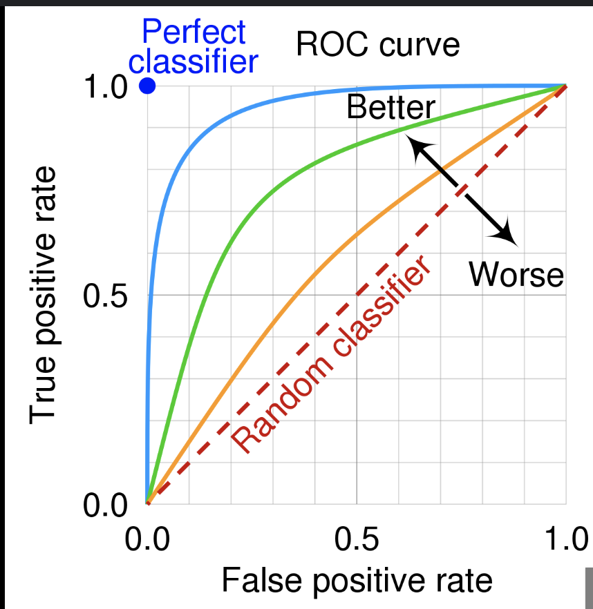
Another important metric is ROC-AUC. The ROC curve plots the true positive rate against the false positive rate as the classification threshold varies. A random classifier gives the baseline diagonal line $y=x$. The AUC is the area under this curve.

AUC can also be interpreted as the probability that the classifier ranks a randomly chosen positive sample higher than a randomly chosen negative sample. It is a useful metric because it accounts for all thresholds and measures how well the model separates the two classes. It is also often useful for imbalanced data, since it depends on the relative ranking of scores rather than one fixed threshold.

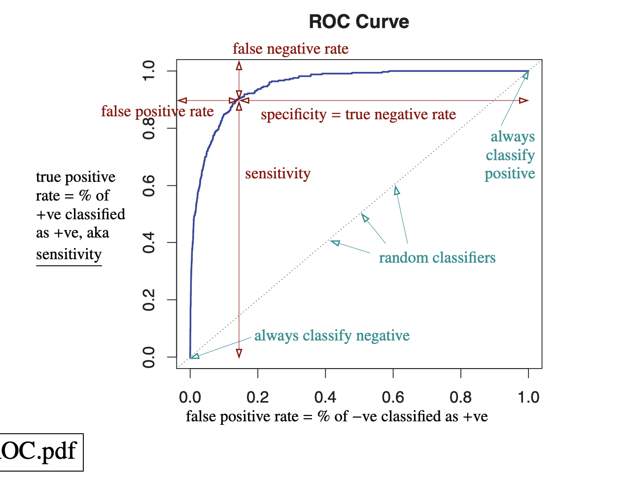ROC and classifiers.	ROC and metrics.

Consider logistic regression for binary classification. It models the log-odds linearly: $$ \log \frac{P(Y=1\mid X)}{P(Y=0\mid X)} = X^\top \beta. $$ Since $P(Y=0\mid X)=1-P(Y=1\mid X),$ this gives $$ P(Y=1\mid X) = \frac{e^{X^\top\beta}}{1+e^{X^\top\beta}}. $$

To fit parameters, we use maximum likelihood. For labels $y_i\in{0,1}$, the likelihood is $$ \prod_{i=1}^n P(Y=y_i\mid x_i,\beta). $$ Taking logs gives $$ \sum_{i=1}^n \log P(Y=y_i\mid x_i,\beta). $$ This can be written as $$ \log P(Y=y_i\mid x_i,\beta)=y_i \log p_i + (1-y_i)\log(1-p_i), $$ where $p_i = P(Y=1\mid x_i,\beta).$ If $y_i=1$, this becomes $\log p_i$, and if $y_i=0$, this becomes $\log(1-p_i)$.

Therefore the negative log-likelihood is $$ -\sum_{i=1}^n \Big(y_i \log p_i + (1-y_i)\log(1-p_i)\Big), $$ which is called the logistic loss, or log loss. It is also the binary cross-entropy loss.

Logistic loss is useful for classification when we want not only a label, but also a probability for each class. It penalizes being confidently wrong, so it encourages probabilistic predictions.

In logistic regression, the model is $$ \hat y_i = P(Y=1\mid x_i,w) = \sigma(x_i^\top w), $$ where $\sigma(z)=\frac{1}{1+e^{-z}}$. If we use MSE, the loss is $$ L(w) = \sum_{i=1}^N (y_i-\hat y_i)^2. $$

The issue is that this loss is generally not convex in $w$. Differentiating gives $$ \frac{\partial L(w)}{\partial w} = \sum_{i=1}^N (y_i-\hat y_i)\hat y_i(1-\hat y_i)x_i. $$ Differentiating again, the Hessian is $$ \frac{\partial^2 L(w)}{\partial w^2} = -\sum_{i=1}^N \hat y_i(1-\hat y_i)(1-2\hat y_i),x_i x_i^\top. $$

Now $\hat y_i(1-\hat y_i)\ge 0$, but the factor $(1-2\hat y_i)$ can be $+$ or $-$. In particular, when $\hat y_i>1/2$, we have $1-2\hat y_i<0$, while when $\hat y_i<1/2$, we have $1-2\hat y_i>0$. So the Hessian does not have a fixed sign, which means the MSE objective for logistic regression is nonconvex.

Also, MSE is natural for ordinary regression with Gaussian noise, since it comes from Gaussian MLE. Logistic regression is Bernoulli, so the natural loss is the negative log-likelihood, namely the logistic loss.

MSE stands for mean squared error: $$ \mathrm{MSE} = \frac{1}{n}\sum_{i=1}^n (y_i-f(x_i))^2. $$

It is natural when we assume the model $$ y = f(x) + \epsilon, $$ where the error $\epsilon$ is Gaussian, say $\epsilon \sim \mathcal{N}(0,\sigma^2)$. Under this assumption, the likelihood of the observed data is proportional to $$ \exp\left(-\frac{1}{2\sigma^2}\sum_{i=1}^n (y_i-f(x_i))^2\right). $$ So maximizing the likelihood is equivalent to minimizing $\sum_{i=1}^n (y_i-f(x_i))^2$.

Therefore MSE is commonly used for regression problems, especially when a Gaussian noise model is reasonable.

• Squared error penalizes large errors, since the error is squared.
• MSE is sensitive to outliers.

Relative entropy is another name for KL divergence. For two probability distributions $P$ and $Q$, it is defined by $$ D_{\mathrm{KL}}(P|Q) = \int P(z)\log\frac{P(z)}{Q(z)},dz $$ in the continuous case, or $$ D_{\mathrm{KL}}(P|Q) = \sum_z P(z)\log\frac{P(z)}{Q(z)} $$ in the discrete case.

It measures how different $Q$ is from $P$, or how much information is lost when we use $Q$ to approximate the true distribution $P$. It is always $\ge 0$, and equals $0$ only when $P=Q$ almost everywhere.

The cross-entropy between $P$ and $Q$ is $$ H(P,Q) = -\int P(z)\log Q(z),dz $$ or in the discrete case $$ H(P,Q) = -\sum_z P(z)\log Q(z). $$ It measures the expected surprise when data are actually generated from $P$, but we evaluate them using $Q$.

The relationship between them is $$ H(P,Q) = H(P) + D_{\mathrm{KL}}(P|Q), $$ where $$ H(P) = -\int P(z)\log P(z),dz $$ is the entropy of $P$.

Intuition:

• $H(P)$ is the intrinsic uncertainty in the true distribution $P$.

• $H(P,Q)$ is the uncertainty we incur when we use $Q$ instead of $P$.

• $D_{\mathrm{KL}}(P|Q)$ is the extra cost / information loss, from using $Q$ to approximate $P$.

Entropy is a measure of randomness or uncertainty in a probability distribution. It can also be interpreted as the average number of bits needed to describe the outcome of a random variable.

If a discrete random variable $X$ takes values $x$ with probabilities $p(x)$, then its entropy is $$ H(X) = -\sum_x p(x)\log_2 p(x). $$

The intuition is that an event with probability $p(x)$ carries information content $ -\log_2 p(x), $ because rarer events are more surprising and require more bits to describe. Entropy is the average of this quantity over all outcomes.

So if the distribution is very concentrated, the entropy is small; if the distribution is more spread out or random, the entropy is large.

SVM uses the hinge loss, $ \max(0,,1-y_i\hat y_i), $ where $ \hat y_i = w^\top x_i + b, $ and $y_i\in\{-1,1\}$. The decision boundary is $ w^\top x_i+b=0, $ and the margin boundaries are $$ w^\top x_i+b=1,\qquad w^\top x_i+b=-1. $$ A correctly classified point with sufficient margin satisfies $ y_i\hat y_i \ge 1, $ so its hinge loss is $0$. If $y_i\hat y_i<1$, then the point is either inside the margin or misclassified, and the loss is positive. So hinge loss penalizes points that are not classified with enough margin.

The objective is to maximize information gain, or equivalently to reduce entropy as much as possible.

If the parent node has entropy $ H(\text{parent}), $ and the split produces child nodes with entropies $ H(\text{child}_1),\dots,H(\text{child}_k), $ then the information gain is $$ \mathrm{Gain} = H(\text{parent}) - \sum_{j=1}^k \frac{n_j}{n} H(\text{child}_j), $$ where $n_j$ is the number of samples in child $j$ and $n$ is the number of samples in the parent node. We compute the entropy before the split, then subtract the weighted average of the entropies after the split. The best split is the one with the largest gain.

$R^2$ can be useful, but it has several limitations:

1. $R^2$ is usually an in-sample metric: it measures how well the model fits the training data, not how well it performs on unseen data. As a result, a model can have a high $R^2$ and still overfit.

2. $R^2$ does not decrease when more predictors are added, even if those predictors are irrelevant $\Rightarrow$ tends to favor more complex models; improvement can be misleading

3. High $R^2$ does not imply that the model is correctly specified, that the predictors are meaningful, or that the model has causal interpretation Inly measures the fraction of variance explained in the sample.

• Fix: adjusted $R^2$ or information criteria such as AIC or BIC.

A bias term lets each neuron shift its activation threshold. Without bias, a layer computes only $ Wx, $ so every decision boundary must pass through the origin. With bias, it becomes $ Wx+b, $ which is much more flexible.

Backpropagation is the algorithm for computing gradients of the loss with respect to all network parameters by repeatedly applying the chain rule from the output layer back to the earlier layers. The idea is to do a forward pass to compute predictions and loss, then do a backward pass to compute gradients, then update the parameters using gradient descent or some optimizer.

Vanishing gradients mean the gradients become extremely small as they are propagated backward through many layers, so early layers learn very slowly. Exploding gradients mean the gradients become extremely large, so training becomes unstable.

They often happen because gradients are products of many Jacobians. Repeated multiplication by numbers $<1$ causes vanishing, while repeated multiplication by numbers $>1$ causes exploding.

Common fixes:

• initialization
• ReLU-type activations
• batch normalization
• residual connections
• gradient clipping
• architectures like LSTM/GRU for sequence models.

No. If all weights are initialized to zero, then all neurons in the same layer produce the same output, get the same gradient, and remain identical during training. The network does not learn different features. We usually use random initialization to break symmetry.

Logistic regression is a single linear model followed by a sigmoid or softmax output. Its decision boundary is linear in the input features.

A DNN stacks many layers with nonlinear activations, can learn nonlinear feature representations. Logistic regression is shallow and linear; a DNN is deep and nonlinear.

Hyperparameter tuning means trying different values of things like learning rate, batch size, number of layers, hidden dimension, weight decay, and dropout rate, then selecting the setting with the best validation performance.

Grid search tries all combinations from a fixed grid. It is simple but expensive for many parameters.

Random search samples hyperparameter combinations randomly from a range or distribution. It is often better in deep learning because only a few hyperparameters usually matter a lot, so random search explores more efficiently.

Dropout randomly sets some neuron outputs to zero during training (but not inference). If the keep probability is $p$, then each unit is kept with probability $p$ and dropped with probability $1-p$.

It works because it prevents neurons from relying too much on specific other neurons, reduces co-adaptation, and acts like a kind of model averaging over many subnetworks.During training, we randomly drop units and usually scale the kept activations by $1/p$ in inverted dropout. During testing, we do not drop units; we use the full network.

Batch normalization normalizes activations within a mini-batch. For an activation $x$, it computes $$ \hat x = \frac{x-\mu_B}{\sqrt{\sigma_B^2+\varepsilon}}, \quad y = \gamma \hat x + \beta, $$ where $\mu_B$ and $\sigma_B^2$ are the batch mean and variance, and $\gamma,\beta$ are learnable parameters.

It helps allow larger learning rates, and adds a small regularization effect through batch noise. During training, it uses the current mini-batch mean and variance. During testing, it uses the running averages accumulated during training.

Sigmoid is $ \sigma(x)=\frac{1}{1+e^{-x}}. $ It maps to $(0,1)$, useful for probabilities, but causes vanishing gradients.

$$ \tanh(x)=\frac{e^x-e^{-x}}{e^x+e^{-x}}. $$ maps to $(-1,1)$ and is zero-centered, but also vanishing gradients.

$$ \mathrm{ReLU}(x)=\max(0,x). $$ cheap to compute, but but neurons can die if they stay in the negative region.

Leaky ReLU: $$ \mathrm{LeakyReLU}(x)=\max(\alpha x,x), $$ with small $\alpha>0$. It keeps a small slope on the negative side, so it helps reduce the dying ReLU problem.

Because without nonlinear activation functions, a multilayer network is still just a linear map. For example, composing $ W_2(W_1x+b_1)+b_2 $ is still affine in $x$. So depth would give no extra expressive power. Nonlinear activations are what let neural networks model complicated nonlinear functions.

SGD: updates parameters using the current gradient only. Simple but noisy and slow.

Momentum: adds an exponential moving average of past gradients, reduces oscillation.

Adagrad: scales each parameter by the accumulated squared gradients, gives larger updates to infrequent features, but learning rate can shrink too much over time.

RMSprop: also uses squared gradients, but with an exponential moving average instead of a cumulative sum, avoids Adagrad’s aggressive decay.

Adam: combines Momentum and RMSprop: keeps moving averages of both the gradient and the squared gradient, then uses bias correction. Default choice to be used.

Batch gradient descent uses the whole dataset for each update. Gradient is accurate and stable, but each step is memory intensive.

SGD or mini-batch SGD uses one sample or a small batch. Each update is cheaper and faster; noise can help escape bad regions, the trajectory is noisier.

Batch size affects this tradeoff. Small batch sizes give noisier gradients but more frequent updates and sometimes better generalization. Large batch sizes give more stable gradients and better hardware efficiency, but they may generalize worse and need careful learning-rate tuning.

If the learning rate is too small, training is very slow and may get stuck for a long time on plateaus.

If the learning rate is too large, updates can overshoot the minimum, oscillate, or diverge; the loss may fail to converge.

A plateau is a region where the loss surface is very flat, gradients are close to zero and optimization moves very slowly. A saddle point is a point where the gradient is zero, but the point is not a local minimum: the function curves upward in some directions and downward in others.

In high-dimensional problems, saddle points are common. They can slow training because first-order methods see very small gradients nearby.

Transfer learning makes sense when we have a pretrained model from a related task or dataset, especially when our own labeled data are limited.

Main idea: Early and intermediate layers may already have useful features, so we reuse them and only fine-tune part or all of the model on the new task. Most useful when the source and target tasks are similar enough that the learned representation transfers.

$k$-modes clustering.