Solving 1d advection equation with a finite volume method
In an effort to clean up files on my computer, I am putting some of the code files on this site to help myself and help others (hopefully, if you find these useful for your projects). These code files are meant to be executable by itself (with appropriate development environments) but tends to be not-so-well documented. More mature code projects will be under the projects page.
In this note, I provide a MATLAB implementation of finite volume method for solving 1d advection equation. Specifically, it is implementing the Lax-Wendroff scheme with MC limiter from LeVeque (Finite Volume Methods), Section 9.5.2 and onwards. This code assumes that the PDE is conservative, which means
\[\partial_t f + \partial_x(u(x)f) = 0\]and is solved with a padding of ng ghost cells on either side of the mesh boundaries. For stability, temporal integration needs the time step to satisfy CFL condition.
function ff = laxWen1d(f, f_ind, nx, v, dx, dt)
    % Takes one time step of 1d conservative advection equation
    %   via lax-wendroff with MC limiter

    % Reference: LeVeque, Randall J. Finite volume methods for hyperbolic problems.
    %   Vol. 31. Cambridge university press, 2002.

    % Input:
    %   f := solution at current times step, (nx+2*ng,1) vector
    %   f_ind := indices of f of non-ghost cells
    %   nx := number of non-ghost cells
    %   v := variable advec. coeff., (nx+1,1) vector
    %        defined on left cell edges (1-1/2):(nx+1/2)
    %   dt and dx are time and spatial step

    % Output:
    %   f0 := (nx,1) solution at next time step on non-ghost cells

    % Positive and negative speeds
    indp = find(v>0); indm = find(v<0);
    vp = zeros(nx+1,1); vm = vp;
    vp(indp) = v(indp); vm(indm) = v(indm);

    % 1st-order right and left going flux differences
    % LeVeque sect. 9.5.2 The conservative equation

    % At cell i: Apdq(i-1/2) = right going  flux = F(i) - F(i-1/2),
    %            Amdq(i+1/2) = left going  flux  = F(i+1/2) - F(i),
    %            where F is numerical flux.
    % Upwind edge flux: F(i-1/2) = vp(i-1/2)f(i-1) + vm(i-1/2)f(i),
    %                   F(i-1/2) = vp(i-1/2)f(i-1) + vm(i-1/2)f(i).

    % Apdq(i-1/2)= F(i) - F(i-1/2),  Amdq(i+1/2) = F(i+1/2) - F(i);
    % F(i-1/2) = vp(i-1/2)f(i-1) + vm(i-1/2)f(i)
    % F(i+1/2) = vp(i+1/2)f(i) + vm(i+1/2)f(i+1)

    % F(i)
    Flux_i = 0;
    % F(i-1/2)
    Flux_m = vp(1:nx).*f(f_ind-1) + vm(1:nx).*f(f_ind);
    % F(i+1/2)
    Flux_p = vp(2:nx+1).*f(f_ind) + vm(2:nx+1).*f(f_ind+1);
    % Apdq(i-1/2) and Amdq(i+1/2)
    Apdq = Flux_i - Flux_m;  Amdq = Flux_p - Flux_i;

    % W = wave with speed u; p = i+1/2, m = i-1/2
    Wp = f(f_ind+1) - f(f_ind); Wm = f(f_ind) - f(f_ind-1);

    % theta's for limiter: LeVeque book sect. 9.13
    % theta_i-1/2 = q(I) - q(I-1) / Wm , I = i-1 v_i-1/2>=0, =i+1 v_i-1/2<0
    % theta_i+1/2 = q(I+1) - q(I) / Wp , I = i-1 v_i+1/2>=0, =i+1 v_i+1/2<0

    % Allocate for limiters
    Thm =  zeros(nx,1); Thp = Thm;

    % At i-1/2
    xsm = indm(indm<nx+1); xsp = indp(indp<nx+1);
    Thm(xsm) = (f(f_ind(xsm)+1) - f(f_ind(xsm)))./Wm(xsm);     % negative speed
    Thm(xsp) = (f(f_ind(xsp)-1) - f(f_ind(xsp)-2))./Wm(xsp);   % positive speed

    % At i+1/2
    xsm = indm(indm>1)-1; xsp = indp(indp>1)-1;
    Thp(xsm) = (f(f_ind(xsm)+2) - f(f_ind(xsm)+1))./Wp(xsm);     % negative speed
    Thp(xsp) = (f(f_ind(xsp)) - f(f_ind(xsp)-1))./Wp(xsp);   % positive speed

    % MC limiter: LeVeque sect. 6.12 TVD Limiters eqn (6.39a)
    phip = max(0,min(min((1+Thp)/2,2),2*Thp));
    phim = max(0,min(min((1+Thm)/2,2),2*Thm));

    % mW = modified wave, LeVeque sect. 9.13 eqn (9.69)
    mWp = phip.*Wp; mWm = phim.*Wm;

    % 2nd-order limited corrections: LeVeque sect. 6.15 eqn (6.60)
    Fp = 0.5*abs(v(2:nx+1)).*(1 - (dt/dx)*abs(v(2:nx+1))).*mWp;
    Fm = 0.5*abs(v(1:nx)).*(1 - (dt/dx)*abs(v(1:nx))).*mWm;

    ff = f(f_ind) - (dt/dx)*(Apdq + Amdq + Fp - Fm);
end
If you save the above code to a file, you can run the following experiments
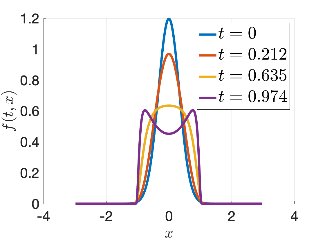
% testing advection with u(x) = x - x^3

% define parameters

% final time
ttf = 1;

% grid size
dy = 0.01;

% spatial grid
yg = (-3:dy:3)';

% number of ghost cells
ng = 2;

% number of effective grid points
ny = length(yg) - 2*ng;

% indexer
idy_f = (ng+1):(ny+ng);
y = yg(idy_f);

% cell centers
ye = [y - dy/2; y(end) + dy/2];

uu = ye - ye.^3;

% refined time step for CFL
dtt = dx/max(abs(uu));
ntt = ceil(ttf/dtt) + 1;
tt = linspace(0, ttf, ntt);
dtt = ttf/(ntt-1);

f = zeros(ny, ntt);

% initial condition
f(:,1) = 3*exp(-0.5*(3*y).^2)/sqrt(2*pi);
for ii = 2:ntt
    tmp = [zeros(ng,1); f(:, ii-1); zeros(ng,1)];
    % take one step
    f(:,ii) = laxWen1d(tmp, idy_f, ny, uu, dy, dtt);
end
You should expect to see the following solutions:
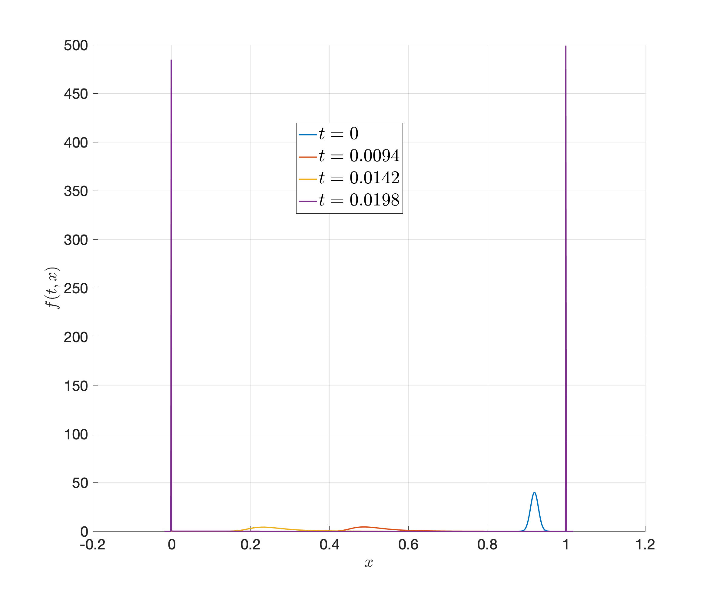
There is another more interesting example where the solution is approximating a fast-changing switch (continuous approximation to indicator). This PDE is very stiff, with \(\Delta t < 10^{-7}\). We provide the code and solutions below.
ttf = .02;
dy = 0.001;
yg = (-0.02:dy:1.02)';

ng = 2;
ny = length(yg) - 2*ng;
idy_f = (ng+1):(ny+ng);
y = yg(idy_f);
ye = [y - dy/2; y(end) + dy/2];

R = 0.0135;  D = 1e-4;
uu = 2*R*(-exp(-20*ye) + exp(-200*ye) + exp(20*(ye - 1))...
    - exp(200*(ye - 1)) - 0.2 ) / D;

dtt = dy/max(abs(uu));
ntt = ceil(ttf/dtt) + 1;
tt = linspace(0, ttf, ntt);
dtt = ttf/(ntt-1);

f = zeros(ny, ntt);
f(:,1) = 1e2*exp(-0.5*(1e2*(y-.9195)).^2)/sqrt(2*pi);
%f(:,1) = 1/(ye(end) - ye(1));

for ii = 2:ntt
    if mod(ii,10000)==0
        disp(ii)
    end
    tmp = [zeros(ng,1); f(:, ii-1); zeros(ng,1)];
    f(:,ii) = laxWen1d(tmp, idy_f, ny, uu, dy, dtt);
end
Enjoy Reading This Article?
Here are some more articles you might like to read next: