Practical Uses of Brownian Motion
A Brownian motion $W_t$ is a function of time with the following fundamental properties:
-
\(W_t\) is continuous; \(W_0 = 0\)
-
For every \(t>0\), \(W_t \sim \mathcal{N}(0,t)\)
-
For any \(s, t\), \(W_{s+t}-W_s\sim\mathcal{N}(0,t-s)\), and is independent of the filtration \(\mathcal{F}_s\) (history up to \(s\))
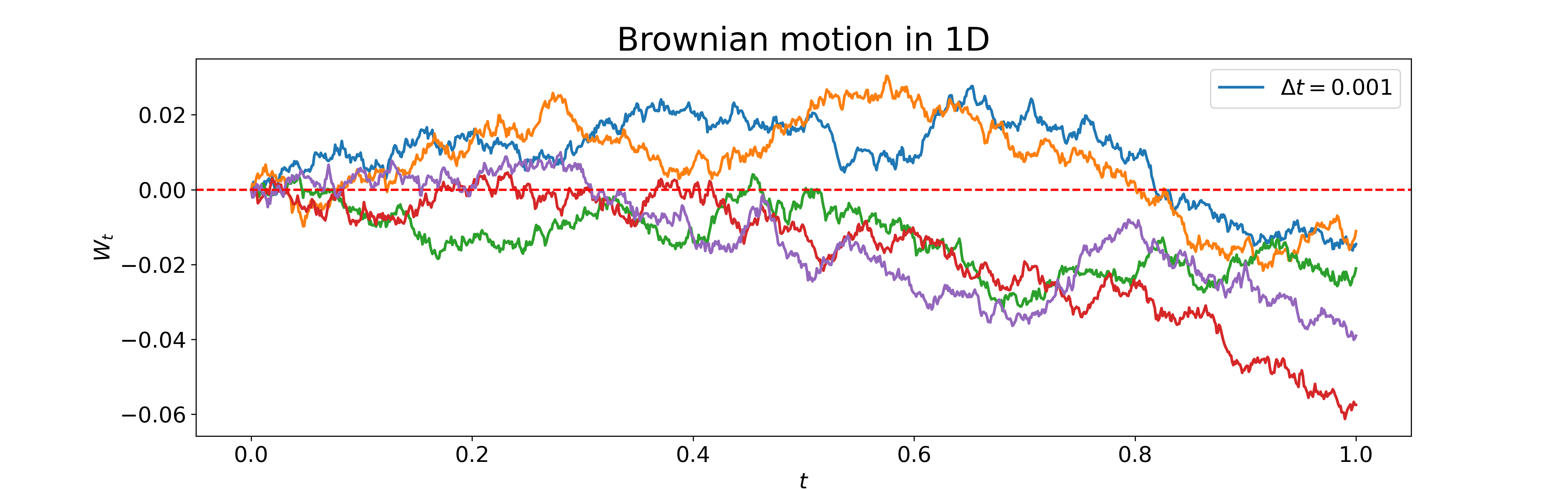
The following is a lovely picture of this process.
Examples of Non Brownian Motions
The following are (unsurprising) answers to the question:
“If a process \(X_t\) satisfies \(X_t\sim\mathcal{N}(0,t)\), and \(t\mapsto X_t\) is continuous, is \(X_t\) a Brownian motion? “
-
Let \(Z\sim \mathcal{N}(0,1)\), define \(X_t := \sqrt{t}Z\)
- This is not a Brownian motion as no additional randomness is introduced at later times. \(X_{s+t}-X_s = (\sqrt{t+s}-\sqrt{t})Z\) is not independent of \(X_s = \sqrt{s}\); their covariance is \(\sqrt{s}(\sqrt{t+s}-\sqrt{s})\).
-
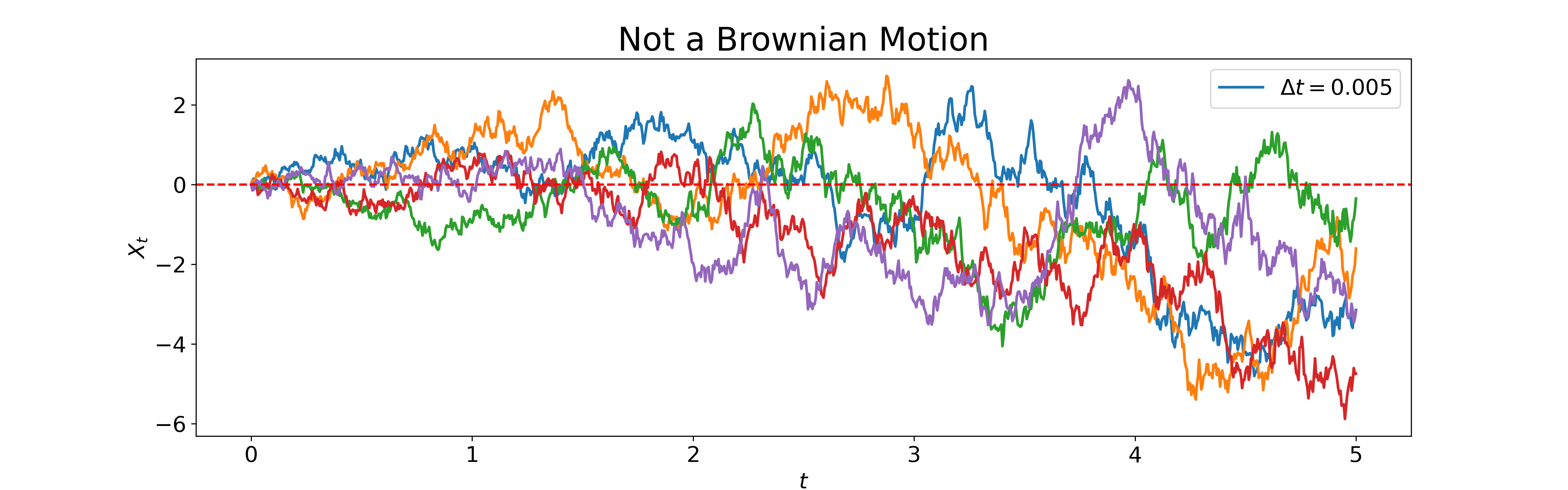
Let \(X_0 = 0\), and:
where \(\sigma_t\) is a deterministic function. We will first solve this equation can show that there is a choice of \(\sigma_t\) such that the process satisfies \(X_t\sim\mathcal{N}(0,t)\).
\[dX_t + \lambda X_tdt = \sigma_t dW_t\]This suggests an integrating factor of \(e^{\lambda t}\). We have:
\[e^{\lambda t}dX_t + \lambda X_te^{\lambda t}dt = e^{\lambda t}\sigma_t dW_t\]Integrating both sides from \(0\) to \(t\), we have:
\[X_te^{\lambda t} - X_0e^{\lambda \cdot 0} = \int_0^t\sigma_s e^{\lambda s}dW_s \Rightarrow X_t = \int_0^t\sigma_s e^{-\lambda(t-s)}dW_s\]The solution is an integral of a deterministic function with respect to standard Brownian motion; we therefore have:
\[X_t \sim \mathcal{N}\bigg( 0, \int_0^t|\sigma_s e^{-\lambda (t-s)}|^2ds \bigg)\]Suppose we want to choose a function \(\sigma_t\), such that:
\[\int_0^t \sigma_s^2 e^{-2\lambda(t-s)} ds = t\]Differentiating both sides, we have:
\[\sigma_t^2 e^{2\lambda t} = e^{2\lambda t} + 2\lambda te^{2\lambda t}\]This means \(\sigma_t = \sqrt{1+2t}\). However, \(X_t\) is not a Brownian motion as the increments are not independent of the history. The covariance can be shown to be nonzero. We simulate this process and visualize the increment covariances.
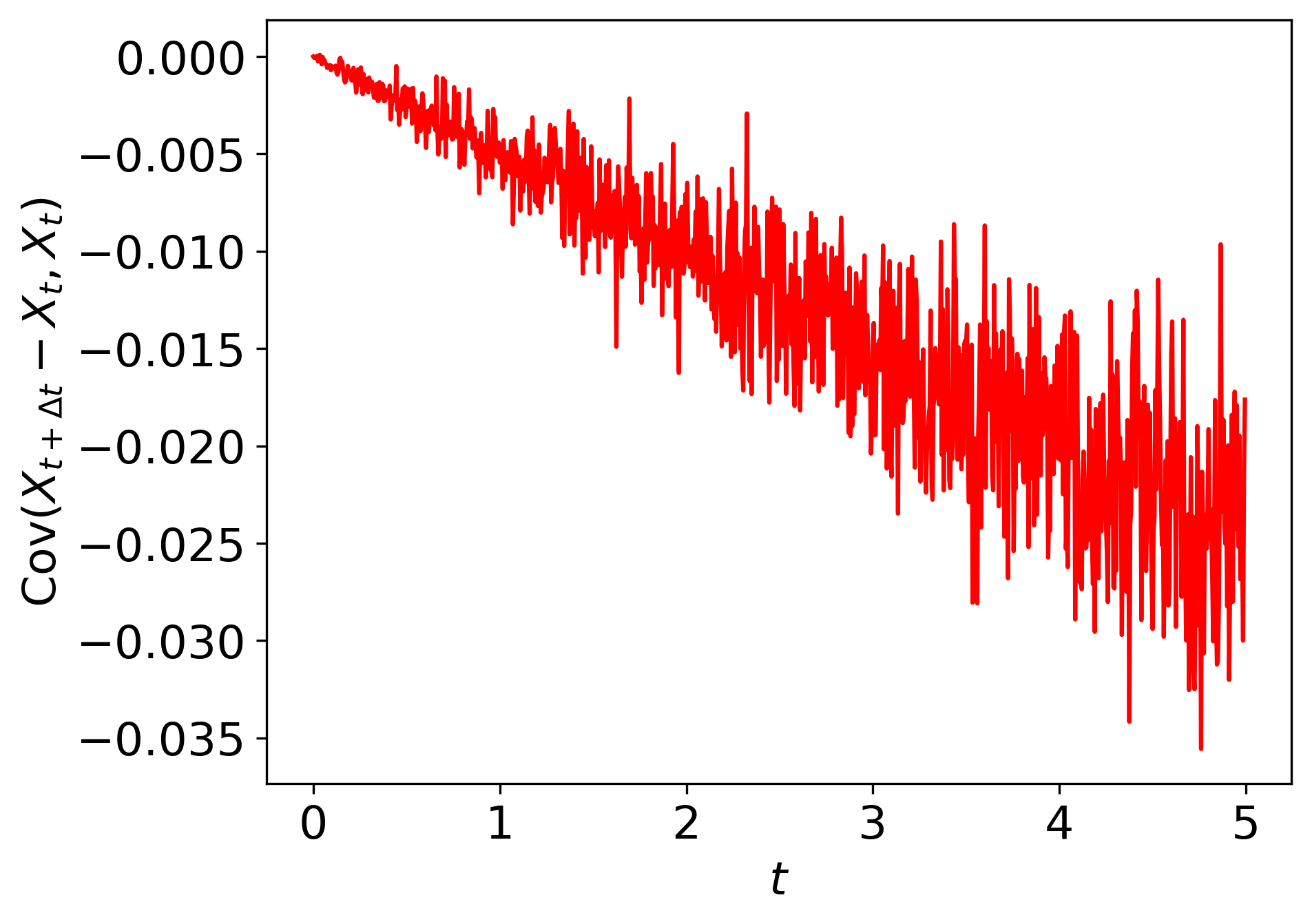
As seen, the estimated (sample size \(N=10^4\)) instantaneous covariance between increments and the past values of \(X_t\) has a slight negative trend as time grows.
Brownian Motion as a Model for Stock Price
We now proceed to discuss obtaining a model for an observed stock price. The following is a plot of the NVDA stock price from 2022 to 2023 (about 252 data points). We notice that the price process is noisy, and seems to have a rather linear trend downwards. The adjusted close price started at $30.07.
Therefore, perhaps the process with a linear trend in time:
\[X_t = \lambda t + \sigma W_t\]can serve the purpose of modeling the price. Suppose we observed the points \(x_0, x_1, \dots, x_n\) at equidistant points \(t_0 < t_1 < \cdots < t_n\), with \(t_{i+1}-t_{i} = \Delta t\), we have:
\[X_{i+1} - X_i = \lambda \Delta + \sigma (W_{i+1}-W_i) \sim\mathcal{N}(\lambda\Delta t, \sigma^2\Delta t)\]and all the increments are independent thanks to the property of Brownian motion. Therefore, we may compute the increments of the price process \(\Delta X_i = X_{i+1} - X_i\), and find the parameters \(\mu,\sigma\) through maximizing the following:
\[\mathcal{L}(\mu, \sigma|\{\Delta x_k\}_{k=0}^{n-1}) = \prod_{k=0}^{n-1}\frac{1}{\sqrt{2\pi\sigma^2\Delta t}}\exp\bigg( -\frac{1}{2\sigma^2\Delta t}(\Delta x_i - \mu\Delta t)^2 \bigg)\]Equivalently, we minimize the negative log-likelihood. In this case, the maximizer can be found exactly.
\[\mu = \frac{1}{n}\sum_{k=0}^{n-1}\frac{\Delta x_i}{\Delta t}\] \[\sigma^2 = \frac{1}{n\Delta t}\sum_{k=0}^{n-1}(\Delta x_i - \mu\Delta t)^2\]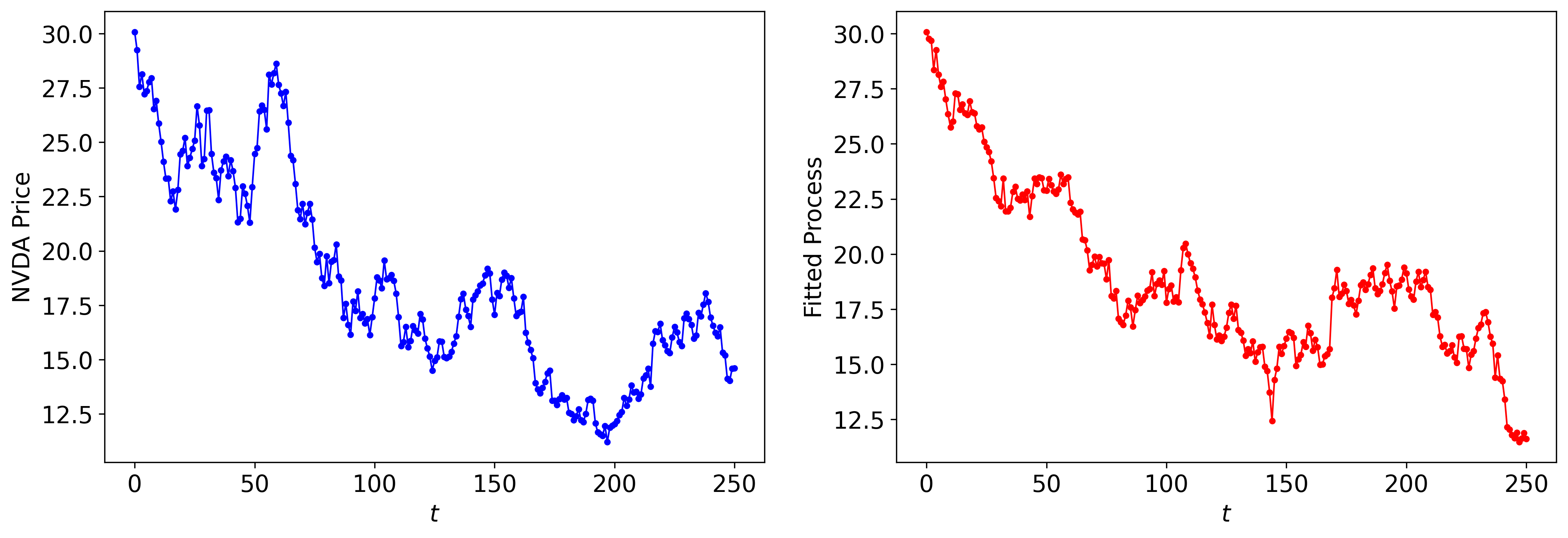
We see that the linear process provides quite a good fit to the data. However, it is not a fundamentally suitable model as in reality, the stock price should never be \(<0\). However, in the process \(X_t\) we have defined, there is always a nonzero probability (and growing to 1, due to the increasing variance of Brownian motion component) of taking on a negative value.
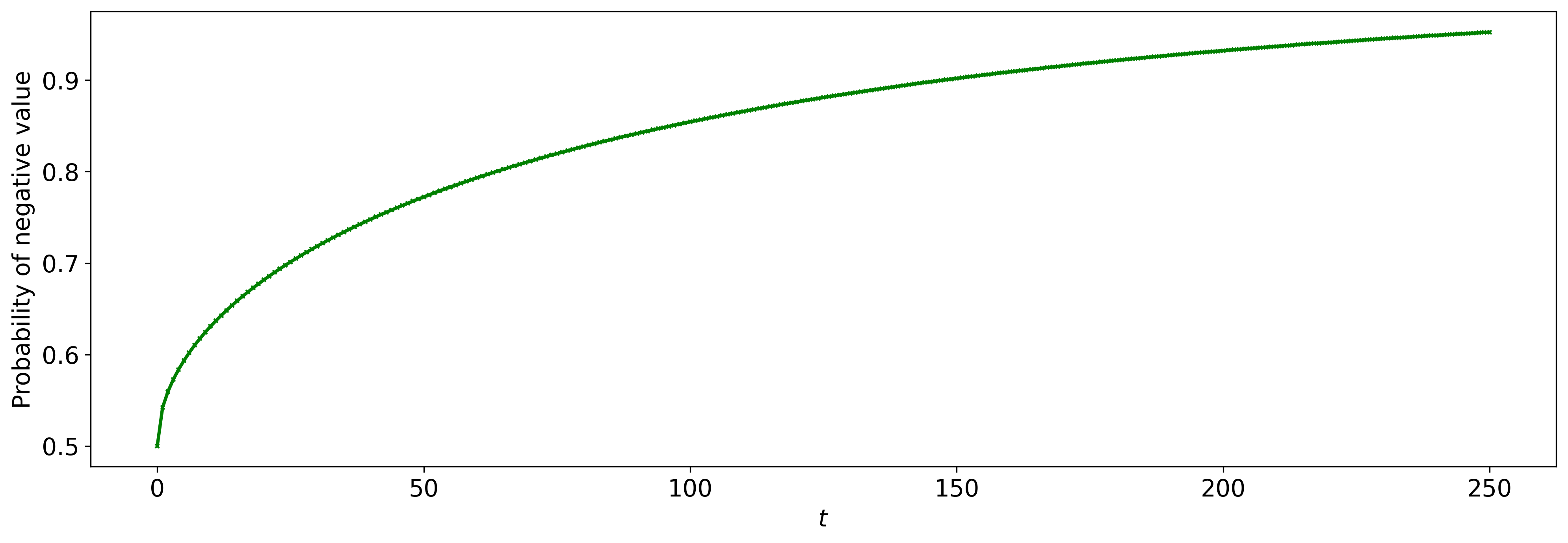
We can compute the following probability explicitly:
\[\begin{align} P(X_t \le 0) &= P\bigg(\frac{X_t - \mu t}{\sigma\sqrt{t}} \le -\frac{\mu}{\sigma}\sqrt{t}\bigg) \\ &= P\bigg(Z\le -\frac{\mu}{\sigma}\sqrt{t}\bigg) \\ &= \Phi\bigg(-\frac{\mu}{\sigma}\sqrt{t}\bigg) \end{align}\]where \(Z\) is a standard normal.