
Reconstructing PDE solutions
Published:
In this short note, we discuss a data-driven viewpoint for reconstructing solutions of reduced partial differential equations arising from stochastic dynamical systems. A representative setting is the evolution of probability densities associated with a dynamical system of the form
\[\begin{cases} \frac{d\mathbf{x}}{dt} = G(\mathbf{x}), \\ \mathbf{x}(0) = \mathbf{x}_0 \sim p_0(\mathbf{x}_0). \end{cases}\]In many applications, one is not interested in the full state distribution, but rather in the evolution of a reduced observable or marginal quantity. This leads naturally to reduced transport-type equations for probability densities. We refer the reader to this page for background on the operator-theoretic perspective.
Reconstruction for homogeneous PDEs
Consider a linear equation of the form
\[\frac{\partial p}{\partial t} - \mathcal{L}_z p = 0,\]with initial condition
\[p(z,0) = p_{z,0}(z), \qquad \lim_{|z|\to\infty} p(z,t) = 0.\]Here \(\mathcal{L}_z\) denotes any linear operator, which is generally assumed to be unknown, and \(p_{z,0}\) is the initial marginal density, assumed either known or estimated from samples, for example by kernel density estimation. In practice, the vanishing boundary condition may be handled numerically by truncating to a sufficiently large computational domain and neglecting rare-event mass outside that domain.
After discretizing in space, the PDE becomes a linear dynamical system
\[\frac{d\mathbf{p}}{dt} = \mathbf{L}_z \mathbf{p}, \qquad \mathbf{p}(0) = \mathbf{p}_z,\]where \(\mathbf{p}(t)\) denotes the discretized density vector and \(\mathbf{L}_z\) is the corresponding discretized operator. The reconstruction task is then to infer an effective linear evolution map directly from data.
Suppose one generates sample trajectories of the underlying stochastic system and uses them to estimate the density snapshots \(\mathbf{p}_0, \mathbf{p}_1, \dots, \mathbf{p}_M\) on a discrete time grid \(t = 0, \Delta t, 2\Delta t, \dots, M\Delta t\). Given \(m < M\) snapshots, define the data matrices
\[\mathbf{X} = \begin{bmatrix} | & | & & | \\ \mathbf{p}_0 & \mathbf{p}_1 & \cdots & \mathbf{p}_{m-1} \\ | & | & & | \end{bmatrix}, \qquad \mathbf{Y} = \begin{bmatrix} | & | & & | \\ \mathbf{p}_1 & \mathbf{p}_2 & \cdots & \mathbf{p}_m \\ | & | & & | \end{bmatrix}.\]A natural least-squares reconstruction problem (which we will refer to as standard reconstruction is
\[\widehat{\mathbf{A}} = \arg\min_{\mathbf{A}} \sum_{i=0}^{m-1} \|\mathbf{p}_{i+1} - \mathbf{A}\mathbf{p}_i\|_2^2.\]The matrix \(\widehat{\mathbf{A}}\) can be interpreted as the best-fit one-step evolution operator for the observed density dynamics.
Example: Kraichnan–Orszag three-mode system
As a first example, consider the Kraichnan–Orszag three-mode problem,
\[\dot{x}_1 = x_1 x_3, \qquad \dot{x}_2 = -x_2 x_3, \qquad \dot{x}_3 = x_2^2 - x_1^2,\]with random initial condition
\[\begin{bmatrix} x_1(0) \\ x_2(0) \\ x_3(0) \end{bmatrix} \sim \mathcal{N} \left( \begin{bmatrix} 0 \\ 0 \\ 0 \end{bmatrix}, \begin{bmatrix} 0.25 & 0 & 0 \\ 0 & 16 & 0 \\ 0 & 0 & 16 \end{bmatrix} \right).\]In a typical experiment, we simulate \(N=3\times 10^4\) random initial conditions up to time \(T=30.0\) with time step \(\Delta t = 5\times 10^{-3}\), and estimate the evolving density using kernel density estimation with a Gaussian kernel and Silverman bandwidth.
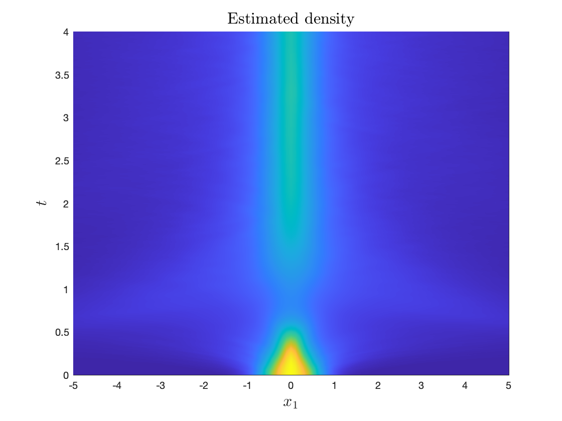
Estimated density \(p(z,t)\) from \(t=0\) to \(t=4\).
Advection- or translation-dominated behavior is known to be challenging for standard linear reconstructions, which often produce oscillatory artifacts or even negative density values. This motivates structure-preserving modifications of the reconstruction procedure.
Orthogonal Proscrustes problem for conservative transport
In the special case where the reduced observable is a coordinate projection \(z = x_k\), the reduced density equation takes the form
\[\frac{\partial p(z,t)}{\partial t} + \frac{\partial}{\partial z} \left[ \mathbb{E}\bigl(G_k(\mathbf{X}) \mid X_k = z\bigr)\, p(z,t) \right] = 0.\]This is a conservative transport equation. In principle, the conditional drift \(\mathbb{E}(G_k(\mathbf{X}) \mid X_k=z)\) may be estimated directly using local regression, moving averages, or smoothing splines, but such procedures require bandwidth or smoothing choices and may be numerically fragile.
Instead, one may attempt to learn the transport dynamics directly from observed density snapshots. However, a naive linear reconstruction typically does not preserve two fundamental properties of a probability density:
- Nonnegativity
- Probability mass conservation
To address this, we may define
\[q(z,t) = \sqrt{p(z,t)}.\]Then \(p = q^2\ge 0\) automatically, and the normalization condition becomes
\[\int_{-\infty}^{\infty} p(z,t)\,dz = \int_{-\infty}^{\infty} q^2(z,t)\,dz = 1.\]Thus, it is natural to reconstruct the dynamics in the variable \(q\) and impose norm preservation. Let \(\mathbf{q}_i\) denote the discretized square-root density snapshots, and define corresponding snapshot matrices \(\mathbf{X}\) and \(\mathbf{Y}\) using \(\mathbf{q}_0,\dots,\mathbf{q}_m\). One may then solve the constrained problem
\[\widehat{\mathbf{M}} = \arg\min_{\mathbf{M}^* \mathbf{M} = \mathbf{I}} \sum_{i=0}^{m-1} \|\mathbf{q}_{i+1} - \mathbf{M}\mathbf{q}_i\|_2^2 = \arg\min_{\mathbf{M}^* \mathbf{M} = \mathbf{I}} \|\mathbf{Y} - \mathbf{M}\mathbf{X}\|_F^2.\]This is an orthogonal Procrustes problem. If
\[\mathbf{X} = \mathbf{U}_r \mathbf{\Sigma}_r \mathbf{V}_r^\top\]is a rank-\(r\) truncated singular value decomposition, then one may project onto the dominant subspace and solve the reduced problem
\[\min_{\widetilde{\mathbf{M}} \text{ unitary}} \|\widetilde{\mathbf{Y}} - \widetilde{\mathbf{M}} \widetilde{\mathbf{X}}\|_F^2, \qquad \widetilde{\mathbf{X}} = \mathbf{U}_r^\top \mathbf{X}, \quad \widetilde{\mathbf{Y}} = \mathbf{U}_r^\top \mathbf{Y}.\]The optimizer is given by
\[\widetilde{\mathbf{M}} = \mathbf{U}\mathbf{V}^\top,\]where \(\mathbf{U}\mathbf{\Sigma}\mathbf{V}^\top\) is the singular value decomposition of
\[\mathbf{U}_r^\top \mathbf{Y}\mathbf{V}_r \mathbf{\Sigma}_r^\top.\]This construction enforces a norm-preserving evolution for \(\mathbf{q}\) and therefore helps maintain physically meaningful reconstructions of the density.
Lagrangian-frame reconstruction for non-homogeneous problems
The homogeneous setting above is only part of the story. In many models, the effective transport velocity is time-dependent, and the resulting dynamics are non-autonomous. In such cases, a single time-invariant linear operator is generally not sufficient to capture the full behavior.
Consider now the advection equation
\[\frac{\partial f_X}{\partial t} + \frac{\partial}{\partial x} \bigl[\mathcal{V}(t,x) f_X(t,x)\bigr] = 0,\]with initial condition
\[f_X(0,x) = g(x),\]together with vanishing boundary conditions, approximated numerically on a sufficiently large domain.
To understand this equation, it is useful to examine its characteristic structure. The associated adjoint equation is
\[-\frac{\partial \widehat{f}_X}{\partial t} - \mathcal{V}(t,x)\frac{\partial \widehat{f}_X}{\partial x} = 0.\]Its solution may be described in terms of the backward flow map \(\Phi(a;X(b),b)\), which evolves a trajectory from time $b$ back to time \(a\). Formally, one may write
\[\widehat{f}_X(0,\Phi(0;X(T),T)) = e^{-T\mathcal{L}_\Phi}\widehat{f}_X(T,X(T)),\]where \(\mathcal{L}_\Phi\) denotes the transport generator along backward characteristics. Equivalently, one may view this as a composition operator,
\[\mathcal{K}u = u \circ \Phi.\]This perspective shows that when the velocity field \(\mathcal{V}(t,x)\) depends explicitly on time, the induced evolution operator must also be time-dependent. A fixed linear reconstruction can therefore be expected to fail in genuinely non-autonomous settings.
This issue also appears in reduced density equations of the form
\[\frac{\partial f_Z}{\partial t} + \frac{\partial}{\partial z} \left[ \mathbb{E}\bigl(G_k(\mathbf{X}) \mid X_k(t)\bigr)\, f_Z(t,z) \right] = 0,\]where the effective drift is generally time-dependent. Even if the original full system is autonomous, reduction can introduce non-Markovian or non-autonomous effects.
A related exact reduced description arises from Mori–Zwanzig projection, where one obtains an equation of the form
\[\frac{dx_k}{dt} = R(x_k(t)) + \int_0^t K(x_k(t-s),s)\,ds + F(t,x_k(0)),\]with random initial condition
\[x_k(0) = X_k \sim g.\]Although the original system may be autonomous, the reduced model typically contains memory terms, and hence is no longer effectively time-invariant. This provides another reason why fixed linear reconstructions often struggle with transient or time-varying behavior.
Test problem: time-dependent advection
As a simple benchmark, consider
\[\frac{dx}{dt} = U \sin(\omega t),\]with random initial condition
\[x(0) = X_0 \sim \mathcal{N}(0,1).\]The density $f_X$ then satisfies
\[\frac{\partial f_X}{\partial t} + U \sin(\omega t)\,\frac{\partial f_X}{\partial x} = 0.\]The corresponding characteristic equation is
\[\frac{d\Phi}{dt} = U \sin(\omega t).\]Suppose we are given snapshots
\[\mathbf{f}_0,\mathbf{f}_1,\dots,\mathbf{f}_{M+1}.\]A standard linear reconstruction seeks an operator $\mathbf{A}$ solving
\[\mathbf{A} = \arg\min_{\widehat{\mathbf{A}}} \sum_{i=1}^{M+1} \|\mathbf{f}_i - \widehat{\mathbf{A}}\mathbf{f}_{i-1}\|_2^2.\]In a representative experiment, one may take \(U=4\), \(\omega={\pi}/{2}\), simulate over \(t\in[0,10]\), and use snapshots up to \(t={5\pi}/{2}\).
For advection-dominated problems, this standard formulation typically performs poorly. Even when it captures part of the transport, it often produces oscillations and struggles with the explicit time dependence of the flow. This motivates two refinements:
- Lagrangian-frame reconstruction, which attempts to reduce oscillations by following the transported structure more closely
- Online updates, which allows the evolution operator itself to vary over time
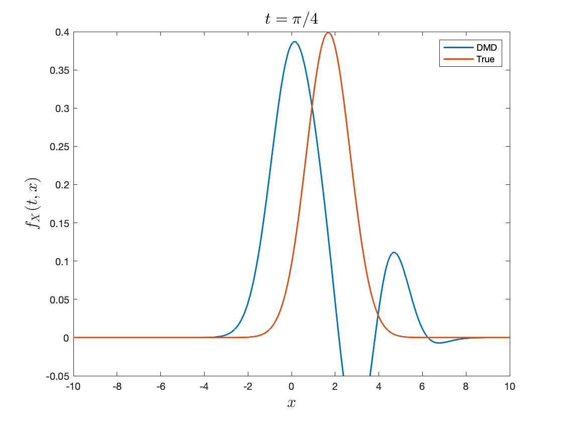
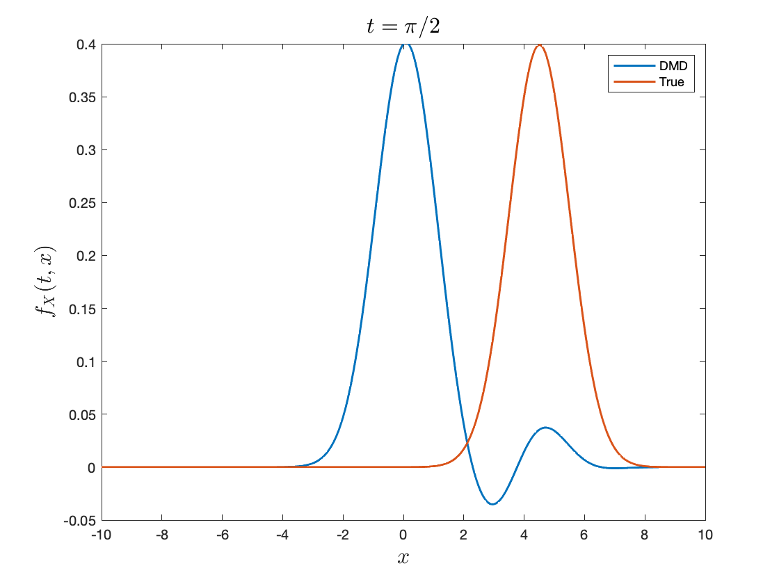
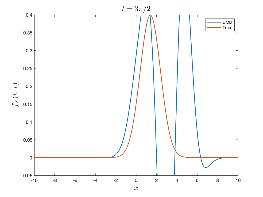
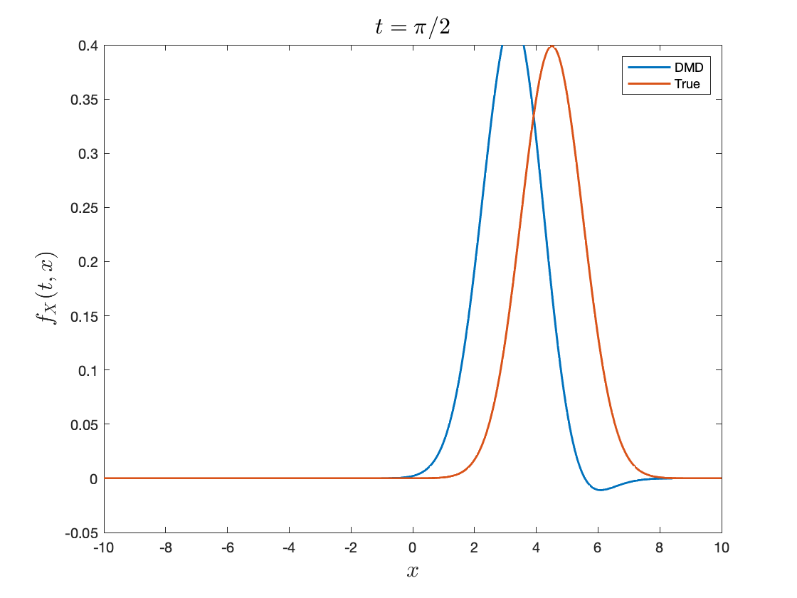
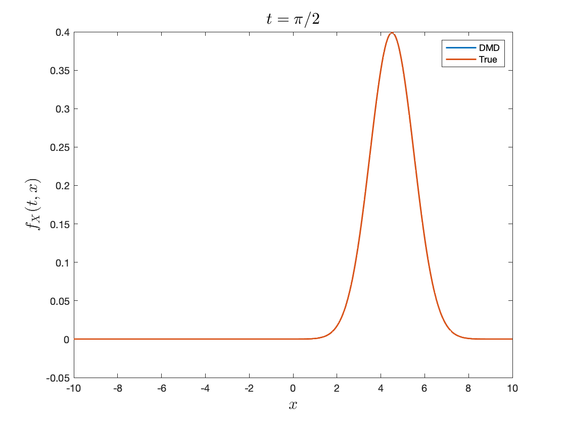
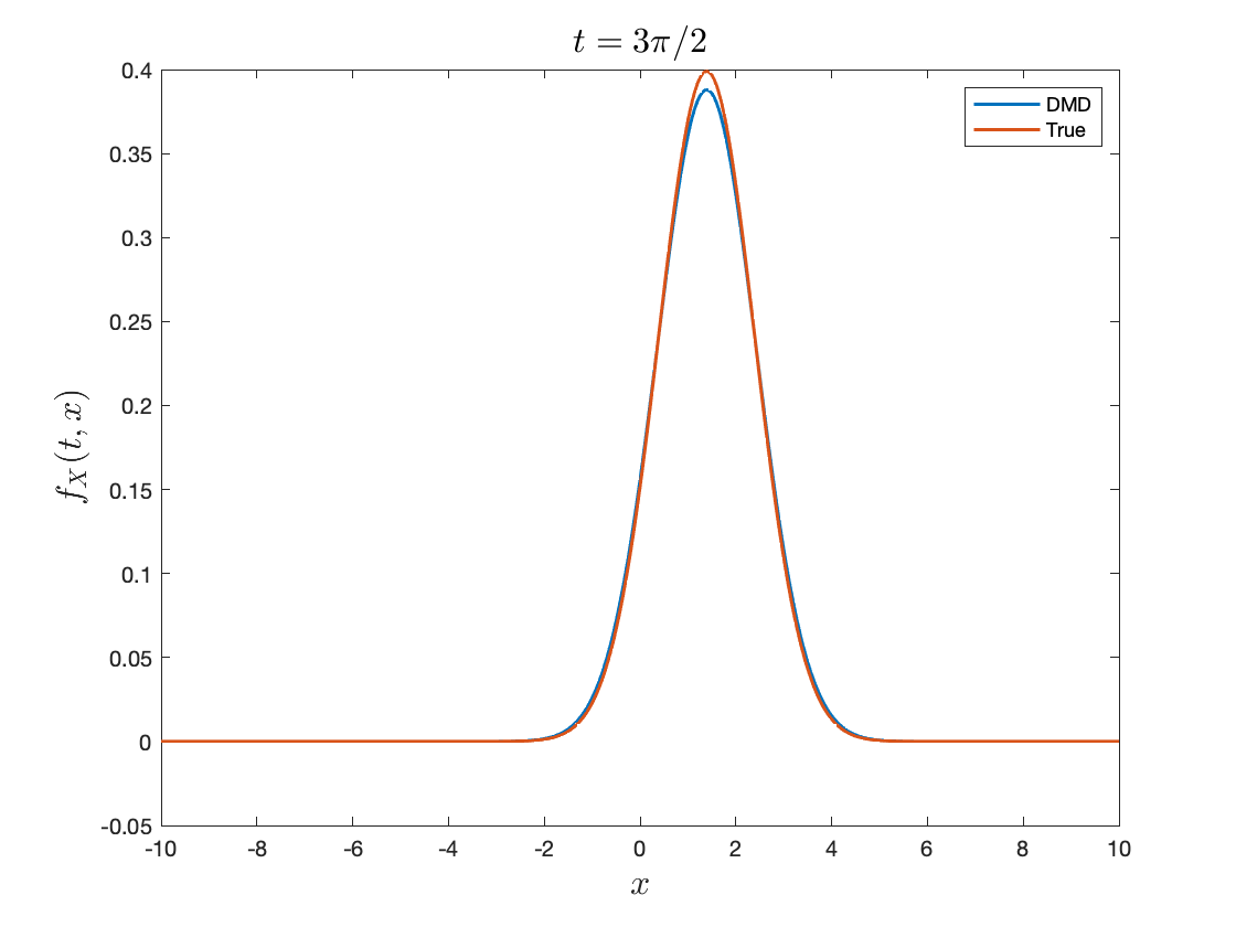
Standard reconstruction fails to reconstruct advection-dominated problems due to the time-invariant assumption. It also exhibits strong oscillations.
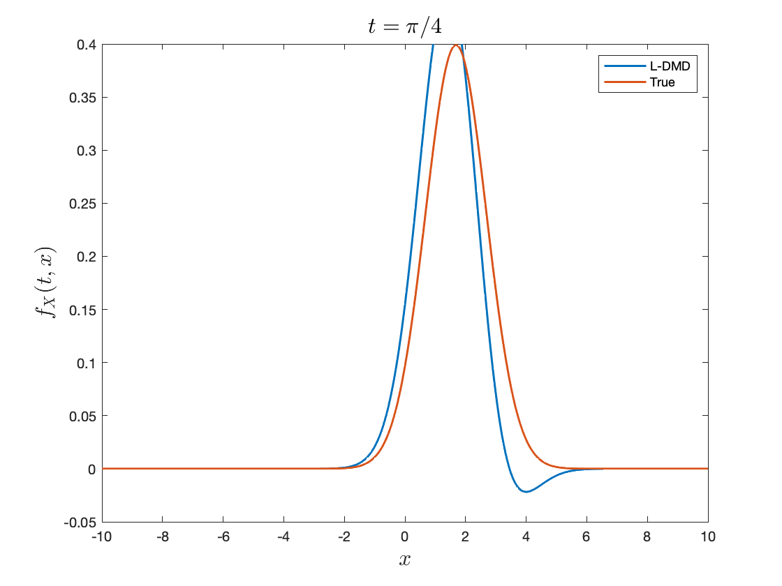
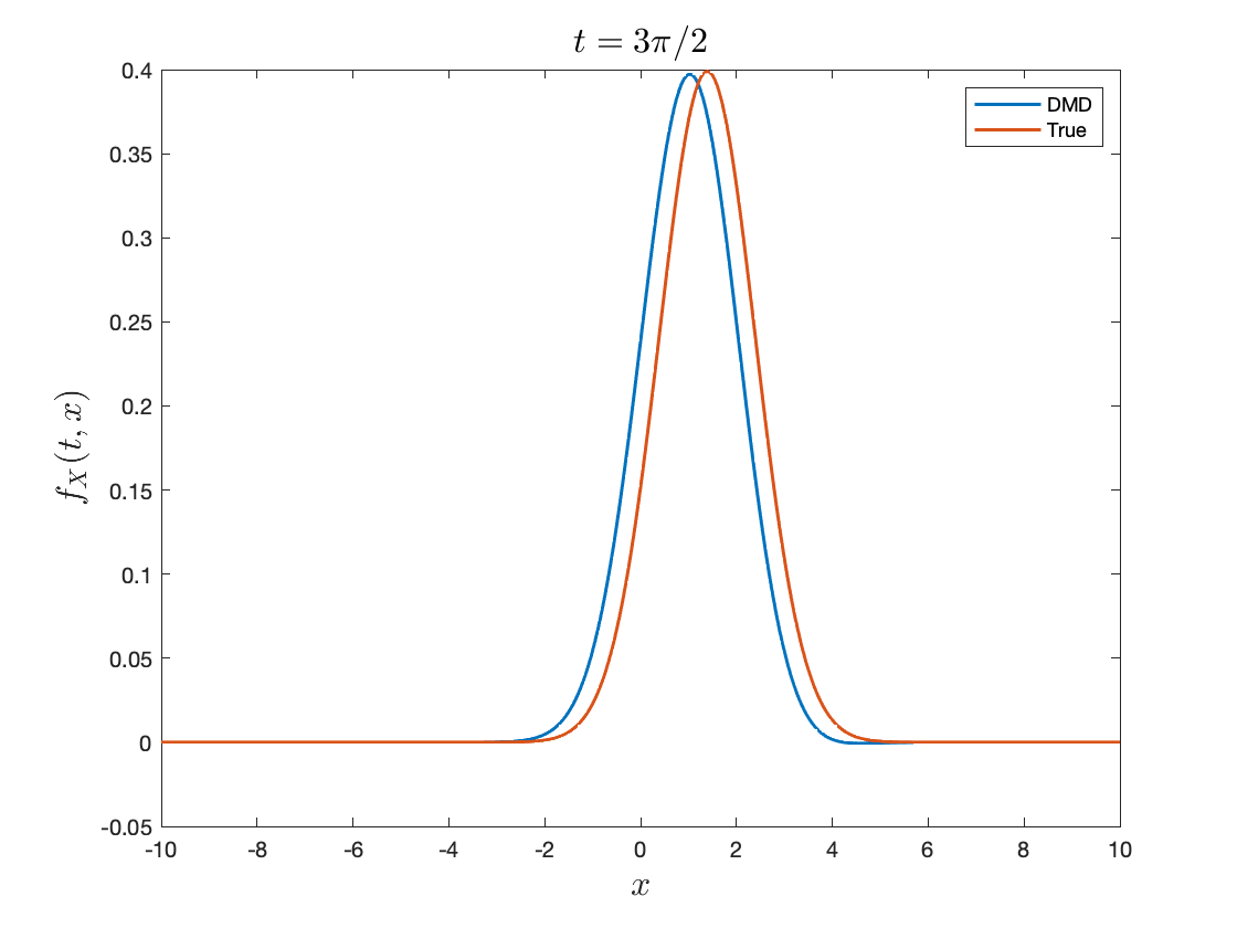
Standard Lagrangian reconstruction shows a grid-tracking effect which reduces oscillations, especially during the first period, but fails due to the inherent assumption of a time-independent operator. Note the periodicity in \(L^2\) error.
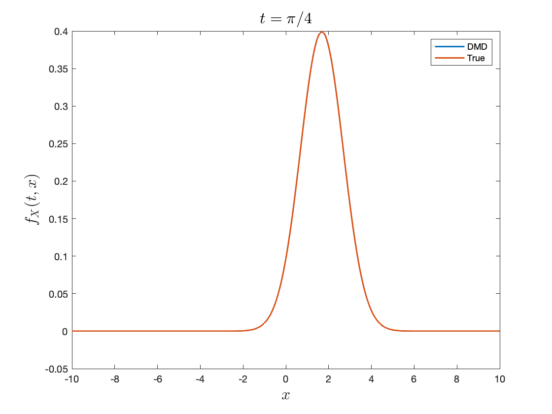
In this case, online Lagrangian reconstruction not only tracks the grid during advection, but also captures time-varying velocity.
Windowed time-dependent reconstruction
To account for time dependence, one may replace a single global operator by a family of local operators defined on time windows. Divide the data into \(J\) windows of size \(m\), with update times indexed by \(n_1,n_2,\dots,n_J\).
Instead of fitting one operator, solve
\[\min_{\mathbf{A}_1,\dots,\mathbf{A}_J} \sum_{i=1}^J \sum_{j=1}^{m} \| \mathbf{f}_{n_i-j+1} - \mathbf{A}_i \mathbf{f}_{n_i-j} \|_2^2.\]The key difference is that the operator is now allowed to vary across time intervals. This is a simple way to encode non-autonomous behavior in the reconstruction.
For a given window \(k\), the least-squares solution is
\[\mathbf{A}_k = \mathbf{Y}_k \mathbf{X}_k^\top (\mathbf{X}_k \mathbf{X}_k^\top)^{-1}.\]Now suppose a new observation pair $(\mathbf{x},\mathbf{y})$ arrives. The updated operator becomes
\[\mathbf{A}_{k+1} = (\mathbf{Y}_k\mathbf{X}_k^\top + \mathbf{y}\mathbf{x}^\top) (\mathbf{X}_k\mathbf{X}_k^\top + \mathbf{x}\mathbf{x}^\top)^{-1}.\]This is a rank-one update of the previous problem, so the inverse may be updated efficiently using the Sherman–Morrison formula,
\[(\mathbf{Q}_k + \mathbf{x}\mathbf{x}^\top)^{-1} = \mathbf{Q}_k^{-1} - \frac{ \mathbf{Q}_k^{-1}\mathbf{x}\mathbf{x}^\top \mathbf{Q}_k^{-1} }{ 1 + \mathbf{x}^\top \mathbf{Q}_k^{-1}\mathbf{x} }, \qquad \mathbf{Q}_k := \mathbf{X}_k\mathbf{X}_k^\top.\]Defining also
\[\mathbf{P}_k := \mathbf{Y}_k\mathbf{X}_k^\top,\]one obtains an online update rule for \(\mathbf{A}_{k+1}\) that avoids recomputing the full pseudoinverse from scratch. A convenient formulation is
\[\begin{cases} \mathbf{z}_{k+1} = \mathbf{Q}_k^{-1}\mathbf{x}, \\[0.5em] \mathbf{w}_{k+1} = \mathbf{A}_k \mathbf{x}, \\[0.5em] \mathbf{A}_{k+1} = (\mathbf{A}_k + \mathbf{y}\mathbf{z}_{k+1}^\top) - \frac{1}{1+\mathbf{x}^\top \mathbf{z}_{k+1}} \left( \mathbf{w}_{k+1}\mathbf{z}_{k+1}^\top + (\mathbf{z}_{k+1}^\top\mathbf{x})\,\mathbf{y}\mathbf{z}_{k+1}^\top \right). \end{cases}\]Computing this update requires \(O(n^2)\) operations when \(\mathbf{A}_{k+1}\in\mathbb{R}^{n\times n}\), whereas recomputing the full least-squares solution directly typically costs \(O(n^3)\). If one processes \(r\) new samples at once, the corresponding cost is \(O(rn^2)\). In rank-deficient settings, an SVD truncation to rank \(k\le n\) can further reduce the effective cost to \(O(rk^2)\), aside from the cost of forming the truncated SVD itself.
Discussion
The main message is that reconstruction of reduced PDE solutions is closely tied to structural properties of the underlying transport equation.
- For homogeneous problems, a fixed linear operator may provide a useful model.
- For probability densities, preserving positivity and mass is essential, which motivates square-root formulations and orthogonal reconstruction.
- For non-homogeneous or time-dependent problems, a time-invariant operator is often too restrictive, and one should instead consider Lagrangian or online time-dependent reconstructions.
Directions
Structure-preserving reconstruction for densities. Reconstruction methods that preserve nonnegativity, mass, and other physical or probabilistic invariants by construction.
Time-dependent reconstruction for reduced dynamics. Adaptive, or online reconstruction methods for non-autonomous reduced equations induced by projection, closure, or memory effects.
Lagrangian-frame reconstruction for transport-dominated problems. Investigate characteristic-based or hybrid Eulerian–Lagrangian approaches that reduce oscillations in advection-dominated regimes.
Theoretical guarantees. Establish consistency, stability, and error bounds for reconstruction under sampling error, density estimation error, and spatial discretization.
References
Craven, P., and Wahba, G. (1978). Smoothing noisy data with spline functions. Numerische Mathematik, 31(4), 377–403. https://doi.org/10.1007/BF01404567
Ewing, R. E., and Wang, H. (2001). A summary of numerical methods for time-dependent advection-dominated partial differential equations. Journal of Computational and Applied Mathematics, 128(1), 423–445. https://doi.org/10.1016/S0377-0427(00)00522-7
Fu, X., Chang, L.-B., and Xiu, D. (2020). Learning reduced systems via deep neural networks with memory. arXiv:2003.09451. https://arxiv.org/abs/2003.09451
Huhn, Q. A., Tano, M. E., Ragusa, J. C., and Choi, Y. (2023). Parametric dynamic mode decomposition for reduced order modeling. Journal of Computational Physics, 475, 111852. https://doi.org/10.1016/j.jcp.2022.111852
Lu, H., and Tartakovsky, D. M. (2020). Lagrangian dynamic mode decomposition for construction of reduced-order models of advection-dominated phenomena. Journal of Computational Physics, 407, 109229. https://doi.org/10.1016/j.jcp.2020.109229
Lu, H., and Tartakovsky, D. M. (2020). Prediction accuracy of dynamic mode decomposition. SIAM Journal on Scientific Computing, 42(3), A1639–A1662. https://doi.org/10.1137/19M1259948
Lu, H., and Tartakovsky, D. M. (2021). Extended dynamic mode decomposition for inhomogeneous problems. Journal of Computational Physics, 444, 110550. https://doi.org/10.1016/j.jcp.2021.110550
Maltba, T. E., Zhao, H., and Tartakovsky, D. M. (2021). Autonomous learning of nonlocal stochastic neuron dynamics. arXiv:2011.10955. https://arxiv.org/abs/2011.10955
Mojgani, R., and Balajewicz, M. (2017). Lagrangian basis method for dimensionality reduction of convection dominated nonlinear flows. arXiv:1701.04343. https://arxiv.org/abs/1701.04343
Mori, H. (1965). Transport, collective motion, and Brownian motion. Progress of Theoretical Physics, 33(3), 423–455. https://doi.org/10.1143/PTP.33.423
Qin, T., Chen, Z., Jakeman, J., and Xiu, D. (2020). Data-driven learning of non-autonomous systems. arXiv:2006.02392. https://arxiv.org/abs/2006.02392
Schaeffer, H. (2017). Learning partial differential equations via data discovery and sparse optimization. Proceedings of the Royal Society A, 473(2197), 20160446. https://doi.org/10.1098/rspa.2016.0446
Williams, M. O., Kevrekidis, I. G., and Rowley, C. W. (2015). A data-driven approximation of the Koopman operator: Extending dynamic mode decomposition. Journal of Nonlinear Science, 25(6), 1307–1346. https://doi.org/10.1007/s00332-015-9258-5
Wu, Z., Brunton, S. L., and Revzen, S. (2021). Challenges in dynamic mode decomposition. Journal of The Royal Society Interface, 18(185), 20210686. https://doi.org/10.1098/rsif.2021.0686
Zhang, H., Rowley, C. W., Deem, E. A., and Cattafesta, L. N. (2017). Online dynamic mode decomposition for time-varying systems. arXiv:1707.02876. https://arxiv.org/abs/1707.02876
Zhu, Y., and Lei, H. (2021). Effective Mori–Zwanzig equation for the reduced-order modeling of stochastic systems. arXiv:2102.01377. https://arxiv.org/abs/2102.01377
Leave a Comment