Temporal Normalizing Flows

Normalizing flows provide a practical way to learn a probability density and sample from it by pushing forward a simple base distribution (e.g., a standard Gaussian) through an invertible mapping. This post describes a temporal extension—conditioning the flow on time, to model time-dependent densities \(p(t,x)\), with a physics-informed regularization based on a Fokker–Planck equation (FPE).

Motivation

Many stochastic systems are described by an SDE

whose probability density \(p(t,x)\) satisfies the Fokker–Planck equation (in 1D)

In applications, we often care about an observable \(Y_t=\psi(X_t)\) rather than the full state. Learning \(p_Y(t,y)\) directly from data/simulation can be viewed as learning a reduced-order PDF model, which captures uncertainty evolution in a lower-dimensional space and supports downstream tasks such as uncertainty quantification, likelihood evaluation, and sampling.

Normalizing flows

Main objective. Given samples \(\{x_i\}_{i=1}^N\sim p_X\), learn a tractable density model \(p_X(x)\) that supports both evaluation and sampling.

Let \(z\sim p_Z\) be easy to sample (e.g., \(p_Z=\mathcal{N}(0,I)\)). A normalizing flow learns an invertible map

By change of variables,

Equivalently,

Maximum likelihood. Maximizing likelihood is equivalent to minimizing KL divergence up to constants; in practice we minimize negative log-likelihood:

Temporal normalizing flow

A clean and common way to add time is to condition the flow on time: \(x = f_\theta(z;\,t),\qquad z=g_\theta(x;\,t).\)

Invertibility is required in \(x\leftrightarrow z\) for each fixed \(t\). Time is treated as an input/conditioning variable.

Then the time-dependent density model is \(p(t,x;\theta)=p_Z\!\big(g_\theta(x;\,t)\big)\, \left|\det\left(\frac{\partial g_\theta}{\partial x}(x;\,t)\right)\right|.\)

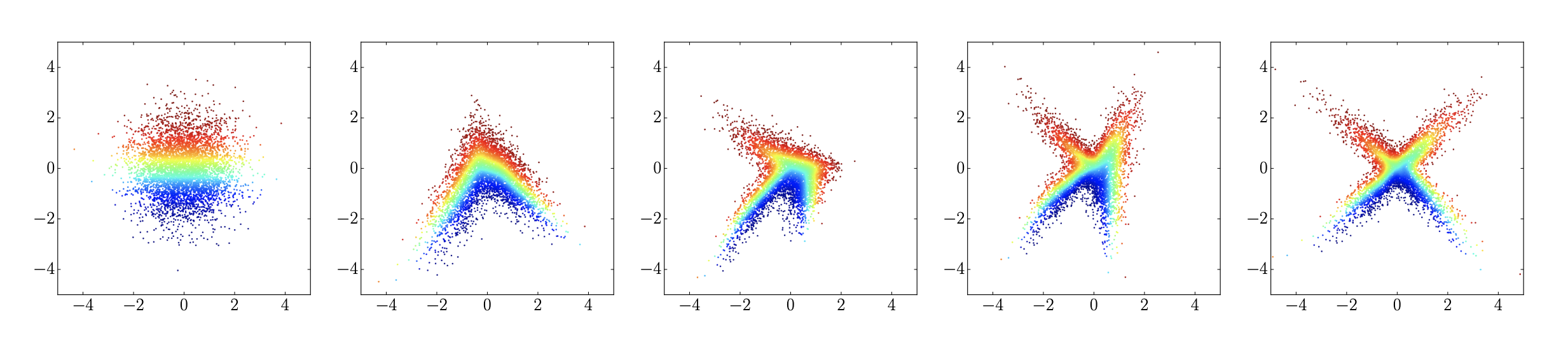
Figure: Flowing samples from a unimodal Gaussian over time (schematic; see Feng et al., 2022).

Physics-informed training via the FPE

If one knows the governing FPE (or want to bias toward an FPE solution), one can add a PDE residual penalty.

Let \(\hat p(t,x)=p(t,x;\theta)\). For diffusion with constant \(\kappa\),

define the residual

Train with a hybrid objective:

$$ \mathcal{L}(\theta) = \mathcal{L}_{\text{NLL}}(\theta)

• \lambda\,\mathbb{E}{(t,x)\sim\Omega}\big[r(t,x;\theta)^2\big]. \(where $\Omega$ defines the spatio-temporal grid; in practice,\)\partial_t \hat p\(and\)\partial{xx}\hat p$$ are obtained by automatic differentiation (e.g., PyTorch autodiff).

This is analogous in spirit to physics-informed neural networks (PINNs), but applied to probability densities and does not have a need to define soft penalties for nonnegativity and mass conservation.

Numerical example: Brownian motion / diffusion

Consider 1D Brownian motion with diffusion coefficient \(\kappa>0\). The density solves \(\partial_t p(t,x) = \kappa\,\partial_{xx}p(t,x).\)

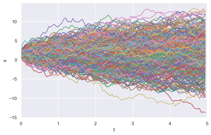
Simulated trajectories

Below is an ensemble of simulated trajectories (Monte Carlo samples):

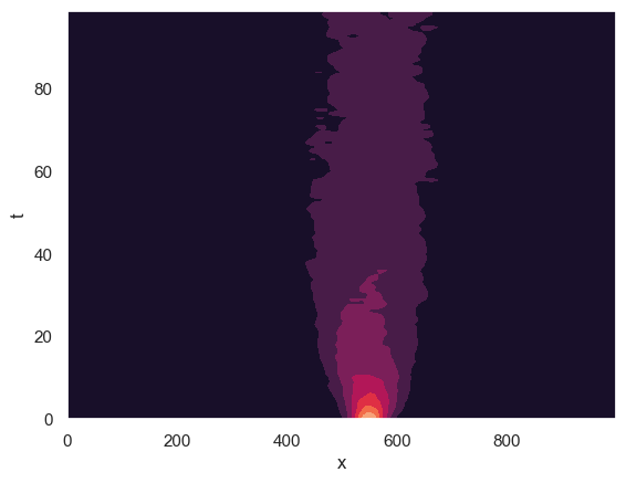
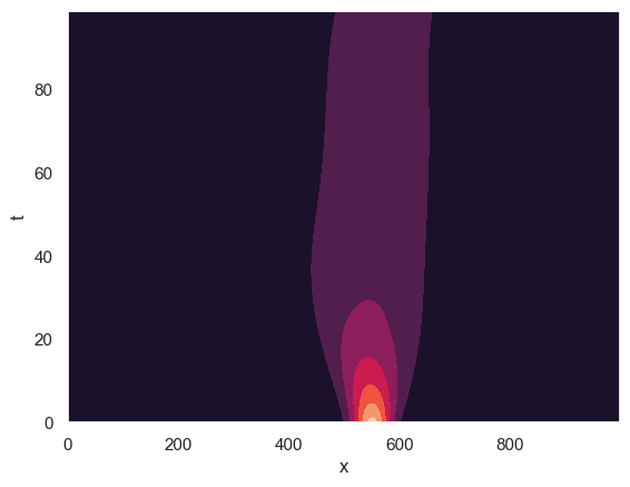
Density estimation: KDE vs temporal NF

A baseline is a time-sliced Gaussian KDE. A temporal normalizing flow learns a smooth \(t\)-conditioned density model:

Directions

A natural next step is to formulate the temporal normalizing flow as a physics-informed density surrogate for time-dependent Fokker–Planck dynamics. Concretely, let \(\hat p(t,x;\theta)=p_Z\!\big(g_\theta(x;t)\big)\left|\det\!\left(\frac{\partial g_\theta}{\partial x}(x;t)\right)\right|,\) where \(g_\theta(\cdot;t)\) is invertible in \(x\) for each fixed \(t\). One may train \(\hat p\) by combining sample-based maximum likelihood with a PDE residual penalty of the form \(\mathcal{L}(\theta) = -\frac1N\sum_{i=1}^N \log \hat p(t_i,x_i;\theta) + \lambda \,\mathbb{E}_{(t,x)\sim\mu}\!\left[\mathcal{R}(t,x;\theta)^2\right],\) where \(\mathcal{R}\) is the Fokker–Planck residual, e.g. \(\mathcal{R}(t,x;\theta) = \partial_t \hat p + \nabla\!\cdot(a\,\hat p) -\frac12 \sum_{i,j}\partial_{x_i x_j}\!\big((BB^\top)_{ij}\hat p\big).\) This provides a competing model for PINNs that claim to solve Fokker-Planck equations.

A second direction is to use this framework for reduced-order PDF methods. Given a low-dimensional observable \(y=\psi(x)\), one may learn a temporal flow model for the reduced density \(\hat p_Y(t,y)\) directly from projected trajectory data, and then test whether \(\hat p_Y\) approximately satisfies a closed effective transport or Fokker–Planck equation in the reduced coordinates. This would turn the temporal flow into a tool for closure discovery.

From a numerical perspective, the key technical questions are: (i) approximation of \(p(t,x)\) and its derivatives by time-conditioned invertible maps, (ii) stability of training under joint likelihood and PDE residual objectives, and (iii) comparison against KDE, histogram-based solvers, and classical Fokker–Planck discretizations in terms of likelihood error, Wasserstein error, and residual consistency. These questions are especially relevant in moderate and high dimensions, where direct grid-based PDF solvers become prohibitively expensive.

References

• Xiaodong Feng, Li Zeng, Tao Zhou. Solving Time Dependent Fokker-Planck Equations via Temporal Normalizing Flow. Communications in Computational Physics, 32(2):401–423, 2022.
• Gert-Jan Both, Remy Kusters. Temporal Normalizing Flows. arXiv:1912.09092, 2019.
• Maziar Raissi, Paris Perdikaris, George Em Karniadakis. Physics Informed Deep Learning (Part II): Data-driven Discovery of Nonlinear Partial Differential Equations. arXiv:1711.10566, 2017.
• Adam Paszke et al. Automatic differentiation in PyTorch. 2017.